Working with the Map
The map control (generally on the right-hand side of the different task screens) is fundamental to the usage of SolarFarmer and is worth getting to know.
Map Toolbar
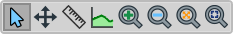
The map toolbar is always present and it's good to get to know the tools. The following tools are present in all the task screens:
| Select | Select individual objects on the map (such as inverters and layout regions).
Press the CTRL keyboard key to select multiple objects. |
|
| Pan & Zoom | Left-click and drag to pan the map. Use the mouse-wheel to zoom in and out. |
|
| Ruler | Left-click once to set one end of a ruler. Move the mouse and left-click to set the other end. The distance (in metres) is shown on the ruler line. Right-click to clear the current ruler. |
|
| Elevation Profile Tool | Shows the profile of terrain elevation between two points. See Elevation Profile Tool for a more detailed explanation of how to use this. |
|
| Zoom in | Instantly zoom in by a fixed amount. | |
| Zoom out | Instantly zoom out by a fixed amount. | |
| Zoom to extents | Zoom the map to the full extents of all objects in the workbook (not including background imagery and elevation data) | |
| Zoom to extents of selected items | Zoom the map to the full extents of all selected objects in the workbook. |
Other tools will appear depending on the current task. The Design Layout task has quite a few!
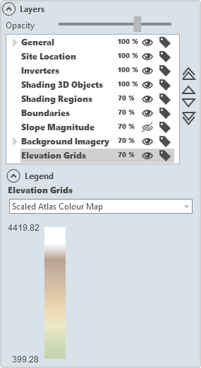
Map Layers
The map is made up of several layers, each responsible for displaying different types of data of the PV plant. You can turn layers on and off and change their opacity to help you to visualise the data better.
The Layers panel is usually minimized in the top-right of the map area:

Just click it to open the Layers panel. It lists the currently available layers (not all are available all the time -- depending on the data you have added to your workbook).
Click the eye icon ( ) to toggle a layer's visibility (the icon becomes
  when the layer is invisible).
Click the tag icon ( ) to toggle the visibility of the labels on a layer (the icon becomes
  when the labels are invisible).
Select a layer and slide the Opacity slider (at the top) to change the layer's opacity. 0% means it is fully transparent and thus invisible. 100% means it is fully opaque and you won't see any other layers below.
Clicking on the triangular arrow buttons on the right move selected layers up or down. The layers are rendered bottom-up, so any layers near the top will be rendered last and thus 'on-top' of the others. Generally big layers that take up the whole area (such as background imagery and elevation grids) are at the bottom so that smaller objects (such as inverters and shading objects) are visible on top of them.
There is a Legend area that becomes visible and available when certain map layers are selected. Important for the Elevation Grids map layer to change the colour scheme from a range of options.
Slope Magnitude Layer
When you import terrain into the SolarFarmer workbook a Slope Magnitude layer is automatically calculated and added:
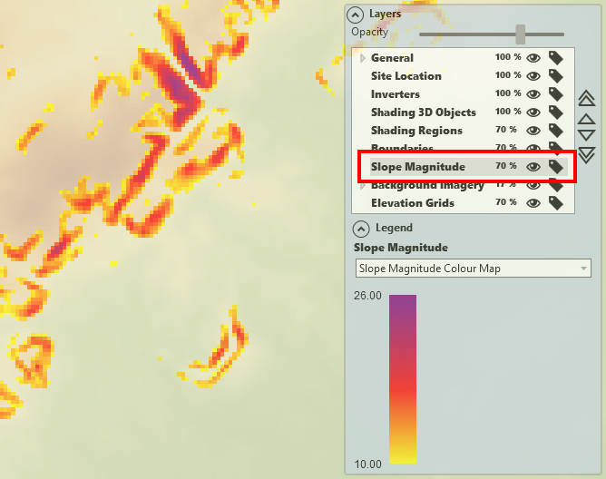
This helps to highlight areas of the terrain with large slopes so that when laying out a new site it is easier to avoid high-slope areas. Turn the visibility of this layer off if you do not wish to view it.
3D Mode
The map has a 3D mode to enable you to see the terrain and objects in 3D, to help visualise the site closer to as it will be in real life.
Click on the '3D' button at the bottom of the map area to switch the view to 3D.

Note that only the area that is currently visible in the 2D map will be portrayed in 3D.
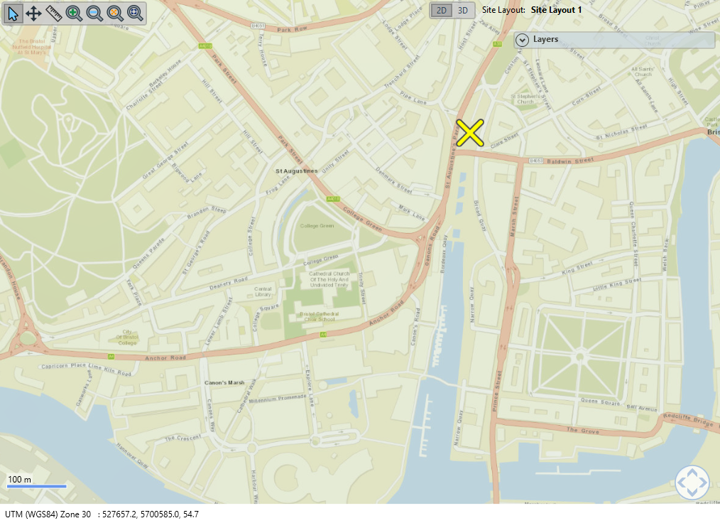
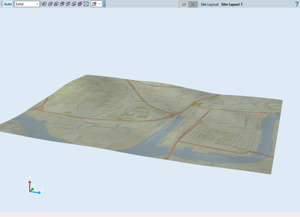
See for example a close-up of the city of Bristol, UK below. When you switch to 3D only the 3D terrain in that close-up area will be visible in 3D. It takes a screenshot of whatever layers are visible in 2D mode to drape over the terrain:
 |
 |
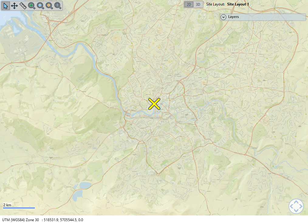
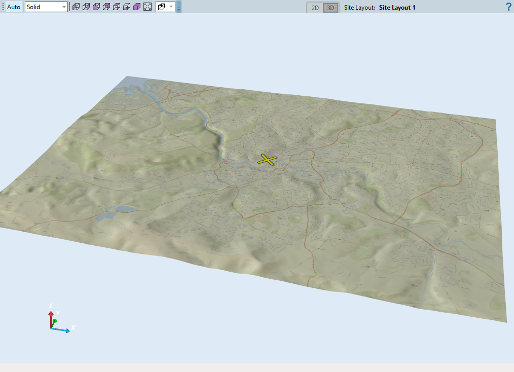
If you go back to 2D mode (press the '2D' button at the bottom of the map) and zoom out. Then go back to 3D view, you will see that a wider area is now portrayed in 3D:
 |
 |
Click on the Help question mark button ( ) in the top-right of the 3D view to show mouse and keyboard controls for working in the 3D view. It may take a while to get used to them.
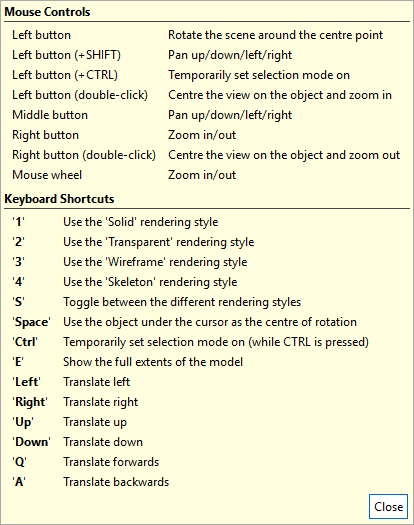
The main useful one to know is to double-click with the left mouse button on the point you wish to rotate around.
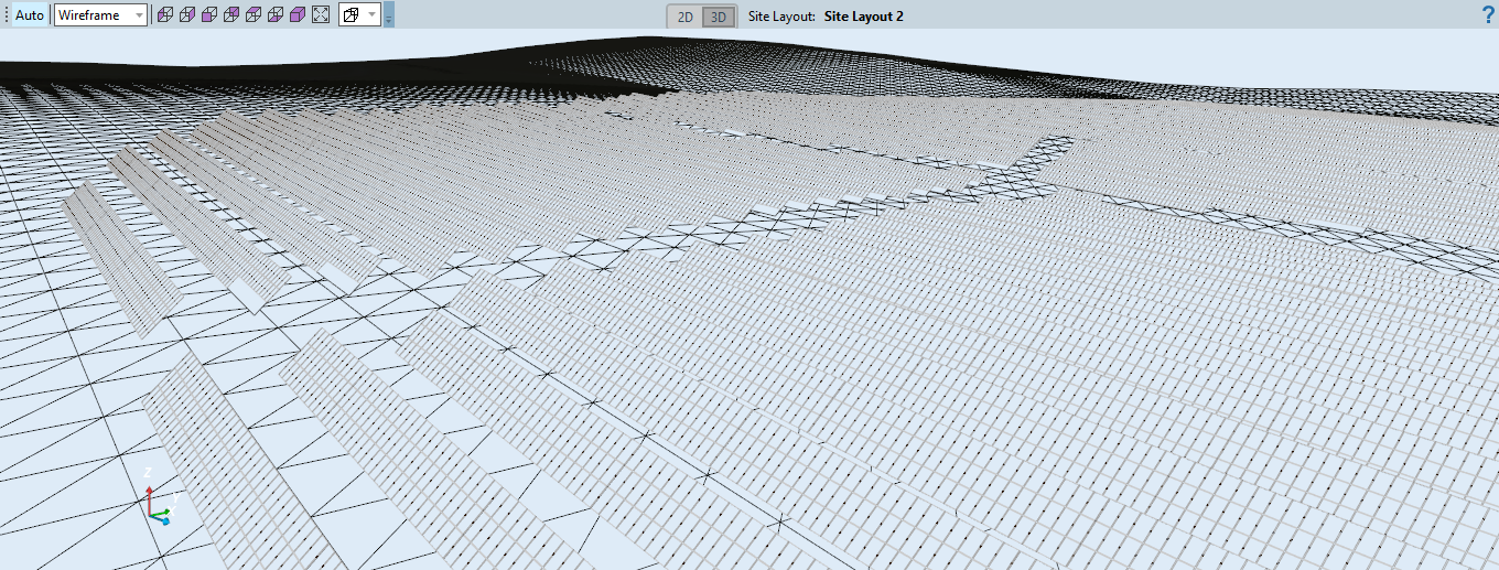
Changing the rendering mode to Wireframe can be useful to see individual modules and get a better feel for the undulating terrain. Change the rendering mode with the drop-down in the top-left (or use the keyboard shortcuts):
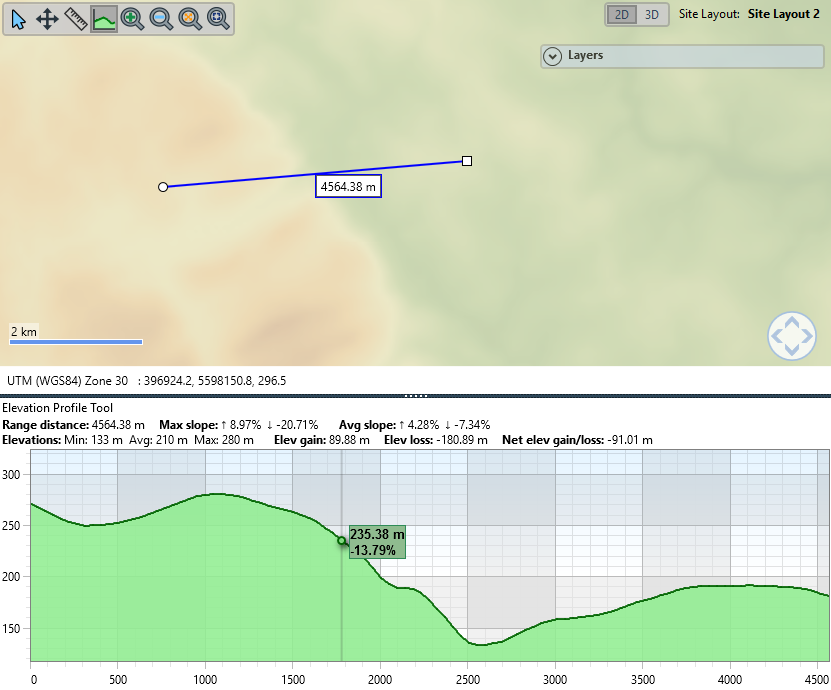
Elevation Profile Tool
With this tool selected, left-click once to set one end of the profile line.
As you move the mouse the profile slope updates on the chart below the map (that has appeared). The distance (in metres) between the start and end of the line is shown on the line in the map. Note that the chart series fills the available space, so the slopes may appear to be steeper/shallower than they are in real-life.
101 sample points are used along the line (so the distance between them depends on the length of the line), sampling the elevation at each point.
Left-click to set the other end of the profile line. Various statistics relating to the elevation profile are shown above the chart:
The total distance of the line (in metres)
The maximum uphill and downhill slopes (in percentages)
The average uphill and downhill slopes (in percentages)
The minimum, average and maximum elevation (in metres above sea-level)
The total elevation gain along the line (in metres)
The total elevation loss along the line (in metres)
The net elevation gain/loss from the start to the end of the line.
Hovering the mouse cursor over the chart gives you a tooltip containing the elevation and slope at that point: